Pricing European Options using COS Method in Python under GBM

Today, I’m going to propose an alternative method to price a European Option based on the famous COS Method proposed for the first time by Fang and Oosterlee in 2008.

The basic idea besides this method is to replace the risk-neutral probability density (RND) function with its Fourier-cosine series expansion since the coefficients can be derived in an analytical way and depend on the so-called characteristic function (CF).

The COS method is very useful as it is able to price a vector of strike prices at a relatively low computational cost.

import numpy as np
from scipy.stats import norm
from scipy.special import erf
import matplotlib.pylab as plt

Let us suppose we want to price European Call Options with the following characteristics:

1. Spot Price = 100 and the log-price S_t follows a Geometric Brownian motion, i.e., the asset dynamic is described by the following process S_t = mu*S_t*dt + sigma*S_t*dW_t (where W_t is Wiener Process). Moreover, mu and sigma are set as constants as in B&S framework.
2. Strike Prices K= [50,80,100,120,150]. We want to directly price a Deep-OTM, OTM, ATM, ITM and Deep-ITM options.
3. We set the other options’ parameters as follow: the risk free r=0.1, the dividend yield q=0, the maturity of the options tau=0.1, and the realised volatility sigma=0.25
4. The evaluation of the options’ values is done on a truncated interval [a,b] of the log(Price/K). The value of a and b are defined by a combination of a certain constant L (in the paper set as L=10) and the first two cumulants of log-Price distribution. Since the log-Price is normally distributed the first and second cumulants coincide with the first and the second moment, i.e., Cum1 = (mu-0.5*sigma²)dt and Cum2=sigma²*dt. For other models different from the GBM, also the fourth cumulant is take into account, for our purpose it is 0 (Cum4 = 0)
5. Since COS method is based on a numerical approximation we need a suitable N. We will see how the option’s value converges to its reference value as N. Now, set N=32

Since we are dealing with risk-neutral evaluation, we need to transform the mu such that the process is a martingale under the risk neutral measure, i.e., mu = (r-q) — 0.5*sigma².

# Option Parameters
S0 = 100
r = 0.1
q = 0.0
dt = 0.1
sigma = 0.25
K = [50.0,80.0, 100.0, 120.0,150.0]

mu = (r-q) - 0.5*sigma**2

cum1 = (mu - 0.5*sigma**2)*dt
cum2 = sigma**2 * dt
cum4 = 0

L = 10
a = chi1 - L * (np.sqrt(chi2 + np.sqrt(chi4)))
b = chi1 + L * (np.sqrt(chi2 + np.sqrt(chi4)))
N = 32

As I already mentioned, the model is the same one on which Black and Scholes have elaborated the closed formula for the European Option. Thus, we will use the Black and Scholes values as the references.

def StdNormCdf(z):
    phi = 0.5 * (1 + erf(z/np.sqrt(2)))
    return phi

# Black Scholes Model Vectorised
def BlackScholes_Vec(S, K, r, q, dt, sigma, type):
    S = S * np.exp(-q * dt)
    d1 = np.divide((np.log(np.divide(S, K)) + (r + 1/2 * np.power(sigma, 2)) * dt), (sigma * np.sqrt(dt)))
    d2 = d1 - sigma * np.sqrt(dt)
    call  = np.multiply(S, StdNormCdf(d1)) - np.multiply(np.multiply(K, np.exp(-r * dt)), StdNormCdf(d2))
    put  = call + np.multiply(K, np.exp(-r * dt)) - S
    if type == 'call':
        return call
    elif type == 'put': 
        return put

BlackScholes_Vec(S0, K, r, q, dt, sigma, 'call')

OUTPUT: [5.04975083e+01 2.07992263e+01 3.65996845e+00 4.45778141e-02
 5.08421755e-07]

The COS method for European Option Pricing is based on tons of analytical formula. For their derivation, I suggest you refer to Fang (2008). The formula needed to obtain the value of the option is the following:

1. U_k is the cosine-series expansion. It is defined as follow:

where chi_k and psi_k are closed formula developed in various terms in sine and cosine.

2. phi of levy is the characteristic function (CF). It depends on the underlying model assumption, in our case the GBM. It is defined as follow:

The following sections report the code for the evaluation of European Option using the COS method:

# Definition of Chi(c,d) [Equation 22 Fang(2008)]
def CHI(k, a, b, c, d):
    bma = b-a
    uu  = k * np.pi/bma
    chi = np.multiply(np.divide(1, (1 + np.power(uu,2))), (np.cos(uu * (d-a)) * np.exp(d) - np.cos(uu * (c-a)) * np.exp(c) + np.multiply(uu,np.sin(uu * (d-a))) * np.exp(d)-np.multiply(uu,np.sin(uu * (c-a))) * np.exp(c)))
    return chi

# Defintion of Psi (c,d) [Equation 23 Fang(2008)]
def PSI(k, a, b, c, d):
    bma    = b-a
    uu     = k * np.pi/bma
    uu[0]  = 1
    psi    = np.divide(1,uu) * ( np.sin(uu * (d-a)) - np.sin(uu * (c-a)) )
    psi[0] = d-c
    return psi

# Defintion of U_k [Equation 29 Fang(2008)]
def UK(k,a,b,type):
    bma = b-a
    if type == 'put': 
        UK  = 2 / bma * (-CHI(k,a,b,a,0) + PSI(k,a,b,a,0) )
    elif type == 'call':
        Uk = 2 / bma * (CHI(k,a,b,0,b) - PSI(k,a,b,0,b))
    return Uk 

# CF for a GBM
def charFuncBSM(s,r,q,sigma,T):
    phi = np.exp(((r-q) - 0.5 * np.power(sigma,2)) * 1j * np.multiply(T,s) - 0.5 * np.power(sigma,2) * T * np.power(s,2))
    return phi

# Definition of Option Value [Equation 30 Fang(2008)]
def OptionValueCOS1_Vec(S0,K,r,q,dt,sigma,N,a,b,type): 
    bma = b-a
    k  = np.arange(N+1)
    u  = k * np.pi/(b-a)
    V_COS = np.zeros((np.size(K)))
    CFBS = charFuncBSM(u,r,q,sigma,dt)
    for m in range(0,np.size(K)):
        x  = np.log(S0/K[m])
        Term = np.exp(1j * k * np.pi * (x-a)/bma)
        Fk = np.real(np.multiply(CFBS, Term))
        Fk[0]=0.5 * Fk[0] 
        V_COS[m] = K[m] * np.sum(np.multiply(Fk,UK(k,a,b,type))) * np.exp(-r*dt)
    return V_COS

Now, we are ready to test our code and compare the results with the reference value obtained by Black and Scholes closed formula.

print('The values of the option with strike ',K, 'are', OptionValueCOS1_Vec(S0,K,r,q,dt,sigma,N,a,b,'call'), 
      '\nThe Reference Values of BS are: ', BlackScholes_Vec(S0, K, r, q, dt, sigma, 'call'), 
      '\nThe abs errors are: ', abs(OptionValueCOS1_Vec(S0,K,r,q,dt,sigma,N,a,b,'call') - BlackScholes_Vec(S0, K, r, q, dt, sigma, 'call')))

OUTPUT: The values of the option with strike  [50.0, 80.0, 100.0, 120.0, 150.0] 
are [4.95102782e+01 2.07992263e+01 3.65996845e+00 4.45778141e-02 5.08421767e-07] 
The Reference Values of BS are:  [5.04975083e+01 2.07992263e+01 3.65996845e+00 4.45778141e-02
 5.08421755e-07] 
The abs errors are:  [9.87230107e-01 1.78701498e-12 2.39808173e-14 5.16531262e-14
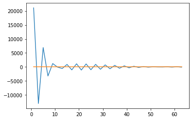
 1.21246325e-14]

As you can observe, N=32 is sufficiently large in order to obtain precise results for our options’ values. However, I decided to simply conduct an analysis of the convergence as N increases for a fixed strike price (K=100). The orange line represents the BS value whereas the blue line is the value using COS method.

Analysis of convergence

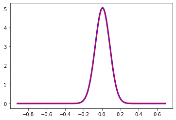
Finally, if we want to recovery the risk-neutral density, the following formula is recovered by Fang(2008):

with F_ks equal to:

The following code implements and displays the risk-neutral density for the log-price, changing maturity to 0.1 and keeping K=100:

def FK(k,a,b,r,q,sigma,T): 
    bma = b-a 
    FK = 2/bma * np.real(charFuncBSM(k*np.pi/bma,r,q,sigma,T) * np.exp(-1j * k * a * np.pi / bma ))
    return FK

def Density(S0,K,a,b,r,q,sigma,T,N): 
    x = np.log(S0/K)
    bma = b-a
    sum = 0.5 * np.cos(0) * FK(0,a,b,r,q,sigma,T)
    for k in range(1,N):
        sum += np.cos(k * np.pi * (x-a)/bma) * FK(k,a,b,r,q,sigma,T)
    return sum

dt = 0.1
mu = (r-q)-0.5*sigma**2
S0 = np.arange(40,200,1)
K = 100
Dens = np.zeros(np.size(S0))
target = np.zeros(np.size(S0))
for i in range(0,len(S0)):
    Dens[i] = Density(S0[i],K,a,b,r,q,sigma,dt,256)
    target[i] = norm.pdf(np.log(S0[i]/K), loc=mu*dt, scale=sigma*np.sqrt(dt))

axis = np.log(S0/K)

plt.plot(axis,Dens, color='blue', linewidth=3  )
plt.plot(axis,target, color='red')

RND for the log-Price

This concludes our article. More difficult models can be involved, e.g. Variance Gamma or CGMY. The only thing to care about is the Characteristic Function that changes among different models Finally, a new alternative approach using COS method will be proposed, without using any underlying model assumption: the so-called iCOS or Implied COS Method, proposed by Evgenii in 2023. But this is another story.

Have a good day, Francesco.